Notes on intelligence, learning & machines 01

A brief
primer on AI

Reading note

A compact map of the ideas behind artificial intelligence: what sits inside what, how machines learn, and what a neural network is actually doing when it trains.

Yellow humanoid robot looking toward the viewer — Personal reference Draft · 2026

02

Before we begin

A map of what we'll cover

AI gets vague quickly. I wanted one reference that follows the thread from “what counts as AI?” to the much less mysterious mechanics of how a neural network learns.

01 / covers

First, untangle the terms

AI, machine learning, neural networks and deep learning are related. They are not interchangeable. We start by putting them in the right order, then compare the three learning setups people usually mean.

02 / follows

Then, follow one training loop

A model makes a prediction. The loss tells us how wrong it was. Backpropagation works out which parameters pushed the answer in that direction, and the optimiser nudges them.

03 / how to read

Use the clicks

The controls are part of the explanation. Click through the comparisons, use the arrows to move between ideas, and open the notes when you want the caveats or sources. The calculus can wait until the appendix.

03

Foundations

So, what actually counts as AI?

Artificial intelligence is a field. The technology inside it keeps changing.

The recurring question is how a machine can do things we associate with intelligence: perceive, plan, decide, communicate, create. Sometimes that means hand-written rules. Sometimes search. Increasingly, it means learning statistical patterns from data. Same umbrella, very different machinery underneath.

1950

The imitation game

Turing asks a practical version of a slippery question: could a machine convince us through conversation?

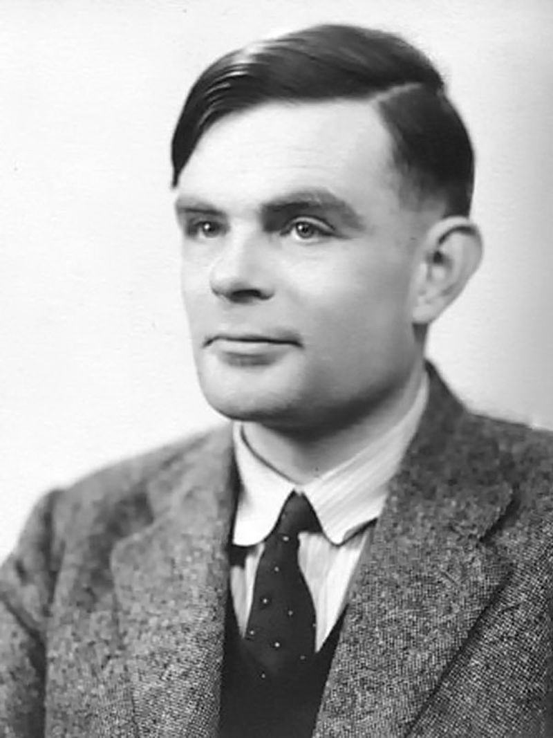
Black-and-white portrait of Alan Turing in 1951 — 1950 Alan Turing

What happened

Turing proposed the “imitation game”: judge the machine by its conversational behaviour, rather than getting stuck arguing about what was happening inside it.

Why it mattered

It turned a beautifully vague philosophical question into something people could test, criticise and try to build toward.

04

The map

The levels of artificial intelligence

Selected / 01

Artificial intelligence

The broad field: machines doing things we associate with intelligence.

Planning · language · robotics

A sensor-equipped robot demonstrator at an aerospace exhibition — Typical use case Robotic perception and task execution

05

Machine learning

Three ways a system can learn

Rows of labelled handwritten digits from the MNIST dataset — Visual example Labelled digits → known classes

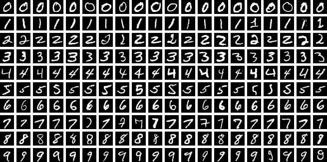
Supervised learning

Give it examples with the answers.

The model makes a prediction, checks it against the labelled answer, then adjusts its parameters so the average error gets smaller. Real systems often mix more than one of these setups.

Input labelled examples

→

Signal prediction error

→

Result mapping to a target

Typical uses

Image classification · spam detection · forecasting

06

Learning with targets

Supervised learning

You show the model the question and the answer.

The input is $x$ . The answer we wanted is $y$ . The model produces $ŷ$ , measures how far off it was, then changes its parameters a little. Repeat this across enough examples and useful patterns begin to stick.

labelled pair
(x, y)→model
ŷ = f(x)→loss
ℓ(y, ŷ)↺

Training objectiveL = (1/n) Σ_i=1ⁿ ℓ(y_i, ŷ_i)Minimise average loss across the training set.

Classification

Which category?

The answer is a category: spam / not spam, one diagnosis among several, cat / definitely not cat.

Binary cross-entropy ℓ = -[y log(ŷ) + (1-y) log(1-ŷ)]

Regression

What continuous value?

The answer is a number: battery life, blood glucose, tomorrow's demand or the price of an asset.

Squared error ℓ = (y - ŷ)²

07

What counts as wrong

Choosing the right loss function

The model cannot optimise “be more correct”. It needs a number.

A loss function turns each mistake into a penalty. The right choice follows the kind of answer we expect and which mistakes should matter most.

01What shape is the answer?A category, a probability or a continuous value?

02Which mistakes cost more?Should one large miss outweigh several small ones?

03How noisy is the data?Should unusual examples dominate the update?

Yes / no target

Binary cross-entropy

−[y log(ŷ) + (1−y) log(1−ŷ)]

Use it when the target is one of two classes and the model outputs a probability. It gives a small penalty to a confident correct answer and a steep penalty to a confident wrong one.

Target: spamŷ = 0.90Small loss

Target: spamŷ = 0.10Large loss

One category among several

Categorical cross-entropy

−log p(correct class)

Use it when the output is a probability distribution across mutually exclusive classes. Training rewards the model for moving probability mass onto the correct category.

car0.12

bicycle · correct0.72

van0.16

Continuous target

Mean squared error

(y − ŷ)²

Use it when the answer is a number and larger misses should matter disproportionately. Squaring makes an error of 20 count sixteen times as much as an error of 5.

Target60

−

Prediction55

→

Squared loss25

Target60

−

Prediction40

→

Squared loss400

Continuous target with outliers

MAE or Huber loss

|y − ŷ| · or · smooth then linear

Use a more robust loss when a few unusual values should not overwhelm the ordinary examples. MAE grows linearly; Huber behaves like squared error near zero and becomes linear for large misses.

08

Learning without targets

Unsupervised learning

There are examples, but no answer key.

That does not mean the system just wanders around. It still needs an objective: make the groups tighter, reconstruct the input more accurately, or find a representation that keeps the useful structure and drops some of the noise.

01 / group

Clustering

Puts similar things near each other.

Market segments · document groups · image regions

02 / relate

Association

Finds things that tend to show up together.

Basket analysis · listening habits · recommendations

03 / compress

Dimensionality reduction

Uses fewer dimensions without throwing away the useful part.

Visualisation · preprocessing · compact representations

09

Learning through action

Reinforcement learning

ObjectiveChoose actions that maximise expected cumulative return.

The feedback comes after an action. Sometimes much later.

The agent learns a policy: a strategy for what to do in a given situation. The awkward bit is that one action changes what happens next. So the useful question is not “Was that move correct?” but “Did this chain of choices lead somewhere better?”

A short trajectory

Try, observe, keep going

A warehouse robot chooses a route, hits congestion and arrives late. That final delay is feedback about the earlier choices too—not just the last turn.

What changes

A strategy, not a lookup table

Across many attempts, actions that tend to produce better long-term outcomes become more likely in similar situations.

10

Optimisation

Training answers two questions: which way, and how far?

The gradient gives us a direction. The learning rate decides how bold to be.

A forward pass produces a prediction and a loss. Backpropagation asks how a tiny change in each parameter would change that loss. Gradient descent then moves the parameters a short distance downhill. Short enough to learn; not so large that we jump straight past the useful bit.

θ_t+1 = θ_t - α ∇L(θ_t)

θ: model parameters
∇L: gradient of average loss
α: learning rate / step size

Important caveat: the gradient only knows the local slope. It is not a map to the best possible solution. Step too far and you overshoot; step too carefully and training takes forever.

Small interactive model · L(w) = w²α = 0.15

Learning rateslowunstable

11

Layered models

Simple behaviour from each neuron gives rise to complex behaviour with many

A deep network is a lot of small calculations, connected and repeated.

One neuron combines its inputs, adds a bias and passes the result through an activation. A layer does many of these calculations at once. Stack the layers and each one gets to work with the patterns found by the one before it.

Start with the small calculation. Then zoom out and see how quickly it becomes a system.

View 01 / one artificial neuron

combine the inputsz = Σ w_ix_i + b

produce an activationa = σ(z)

12

Expressive power

Why activation functions matter

Without them, depth is mostly an illusion.

A layer that only multiplies and adds is an affine transformation. Stack several of them and the algebra still collapses into one affine transformation. The network may be deeper, but it cannot learn a more complicated kind of boundary.

Linear after linear after linear W₃(W₂(W₁x + b₁) + b₂) + b₃ = Ax + c More layers. Still one affine map.

Without an activation

Depth collapses

However many layers we add, the final boundary is still straight.

With a nonlinear activation

Depth compounds

Each activation adds a bend. Stack enough of them and the model can carve out much richer shapes.

13

Expressive power

The small function that stops the whole network being linear

An activation sits between one weighted sum and whatever happens next.

Without a nonlinear activation, stacking layers buys us very little: the whole network still collapses into one linear map. At the final layer, the function also tells us what the output means—a number, a binary probability, or a spread of probabilities across classes.

Hidden-state examples

Output-layer choices

Click the functions. The shape is the point: it determines what gets through and what gets flattened.

Common hidden-layer choice

ReLU

max(0, x)

ReLU turns negative inputs into zero and leaves positive ones alone. That one kink is enough to make the network nonlinear, and it is cheap to compute. The trade-off: a unit can go quiet if it gets stuck on the negative side.

14

Architecture catalogue

Different shapes of data call for different kinds of network

An architecture is a bet about which relationships matter.

Images have neighbourhoods. Sequences have order. Generative models need a way to build rather than only classify. Click a family to see the assumption built into it.

Foundation / fixed-size features

Dense network

Every unit in one layer can contribute to every unit in the next. It is the plainest version of the layered calculation we have already seen.

Input structure: A fixed-length vector of features.
Core move: Learn a weighted connection between every neighbouring pair of layers.
Good for: Structured data, regression and small classifiers.
Current caveat: It ignores space and order unless we encode them into the inputs.

Spatial patterns / shared filters

Convolutional network

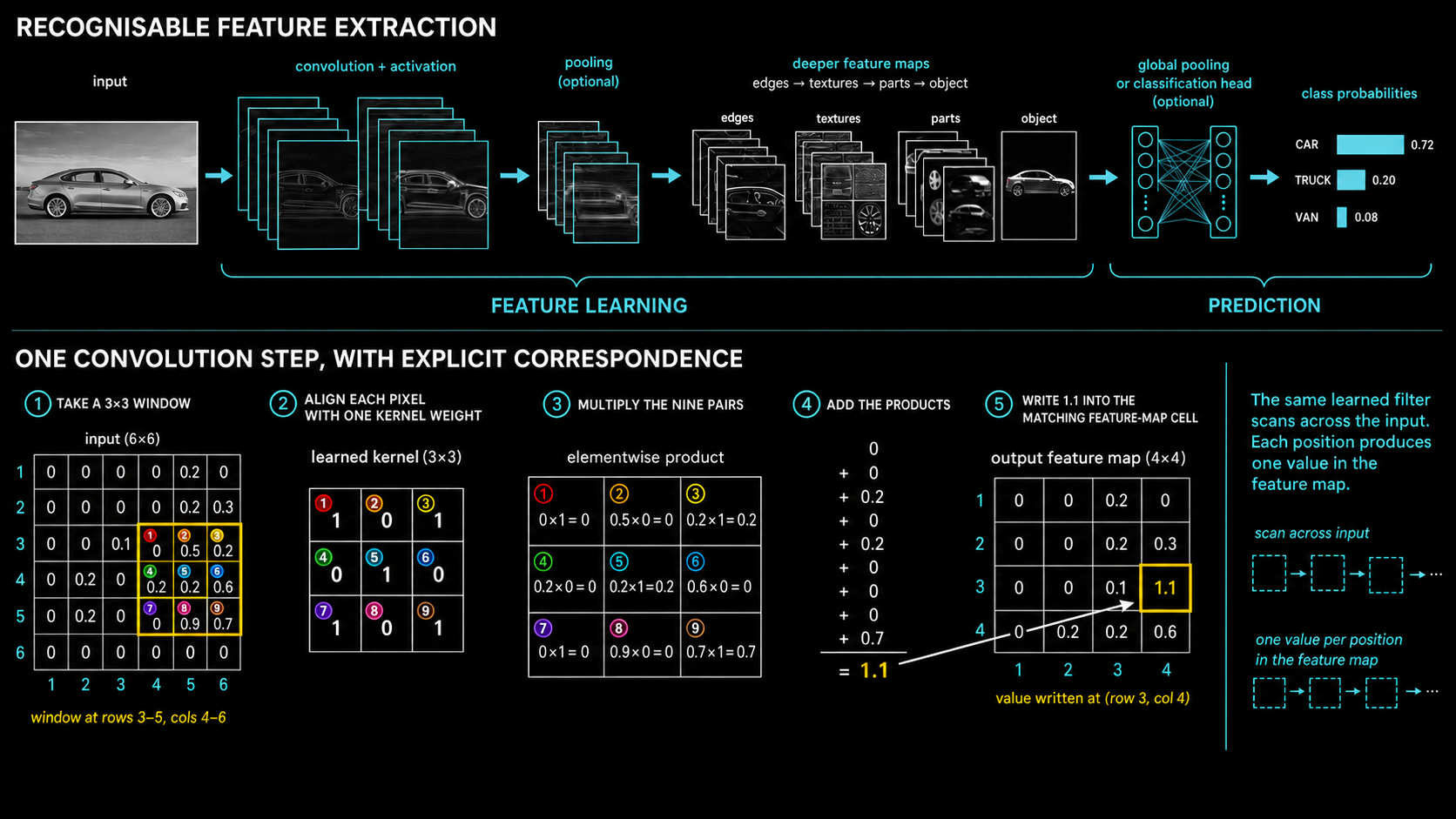
A small learned filter moves across the input. The same detector can recognise an edge or texture wherever it appears.

Open the full visual explainerRecognisable input, feature hierarchy and one mapped convolution step Close visual explainer

A convolutional network follows a recognisable car through edge, texture, part and object feature maps, then maps nine numbered input pixels to a learned kernel, products and the resulting feature-map value 1.1.

Input structure: Grid-like data: pixels, frames or spatial measurements.
Core move: Reuse small learned kernels across nearby positions.
Good for: Image recognition, detection, segmentation and medical imaging.
Current caveat: The local bias is useful, but distant relationships need depth or another mechanism.

Ordered data / shared state

RNN and LSTM

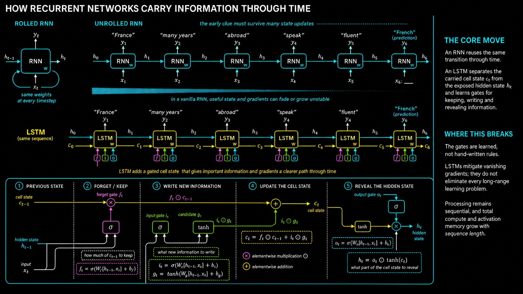
The network carries a hidden state from one step to the next. LSTM gates decide what to write, keep and reveal from that state.

Open the full visual explainerShared recurrent state, the long-range memory problem and one mapped LSTM update Close visual explainer

A recurrent network processes the sequence from France to a prediction of French using shared weights. A parallel LSTM path separates hidden state from cell state, and a detailed cell shows forget, input, candidate and output gates combining into the cell-state and hidden-state updates.

Input structure: An ordered sequence processed one step at a time.
Core move: Reuse the same recurrent weights while passing a state through time.
Good for: Time series, speech and compact sequence models.
Current caveat: Sequential training is slow. Gates mitigate, but do not eliminate, unstable long-range gradients.

Context / attention

Transformer

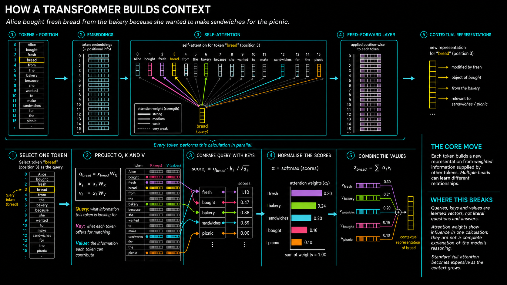
Attention lets each item build its representation from the other relevant items, instead of passing context along one step at a time.

Open the full visual explainerTokens, position, Query-Key-Value projections and one mapped attention calculation Close visual explainer

A transformer converts an Alice sentence into positioned token embeddings, applies query-specific self-attention in parallel, then traces the bread token through Query, Key and Value projections, scaled scores, softmax weights and the weighted sum that produces its contextual representation.

Input structure: Tokens or features, plus information about position.
Core move: Learn which other items each item should attend to.
Good for: Language, multimodal models and long-range context.
Current caveat: Attention can become expensive in memory and compute as the context grows.

Compression / reconstruction

Autoencoder and VAE

An encoder squeezes an example into a smaller latent representation; a decoder tries to reconstruct it. A VAE makes that latent space probabilistic.

Input structure: Examples that can be compressed and reconstructed.
Core move: Learn a bottleneck that preserves enough information to rebuild the input.
Good for: Denoising, anomaly detection, compression and latent generation.
Current caveat: The reconstruction objective may preserve details that are not useful for the real task.

Generation / adversarial training

GAN

A generator tries to make convincing examples. A discriminator tries to spot the fakes. Each model makes the other one harder to fool.

Input structure: Noise or a condition used to seed a generated example.
Core move: Train a generator and discriminator against one another.
Good for: Image synthesis, style transfer, enhancement and augmentation.
Current caveat: Training can be unstable, and the generator can collapse onto too few kinds of output.

Generation / iterative denoising

Diffusion model

Training teaches the model to reverse a gradual noising process. Generation starts from noise and repeatedly turns it into a structured sample.

Input structure: Noise, often paired with text, an image or another condition.
Core move: Learn many small denoising steps that reverse a known corruption process.
Good for: High-quality image, audio and video generation or editing.
Current caveat: Repeated denoising steps cost time and compute, even when faster samplers are used.

15 / 18

Before the notation

The whole training loop, before the calculus

The model makes a prediction. The loss judges it. Backpropagation works out the gradients. The optimiser changes the parameters. The next three slides say the same thing again, just with the notation left in.

01Forward pass
02Loss
03Gradients
04Parameter update

16

Appendix / derivation I

Backpropagation starts at the answer

Before we move backward, keep the useful bits from the journey forward.

01 / keep the weighted input
The weights and bias combine the previous activations into z^ℓ. Save it. Later we need to know exactly where each neuron sat on its activation curve.
02 / keep the activation
The activation function turns z^ℓ into a^ℓ. At the output layer, a^K is the prediction the loss is about to judge.
03 / follow what depends on what
The loss does not see z^K directly. It sees a^K, which depends on z^K. The chain rule says: follow that path and multiply the sensitivities along it.
04 / give the result a name
That sensitivity is δ^K. In plain language: if the output layer's weighted input moved a tiny amount, how much would the loss move?

Click the path to connect prose and notation

Forward / weighted inputz^K = W^Ka^K−1 + b^K

Forward / activationa^K = σ(z^K)

Chain rule / split the path∂L / ∂z^K = ∂L / ∂a^K ⊙ ∂a^K / ∂z^K

Substitute the activation derivativeδ^K = ∇_aL ⊙ σ′(z^K)

Once we have this signal, the output-layer parameter gradients fall out directly.

Bias gradient∂L / ∂b^K = δ^K

Weight gradient∂L / ∂W^K = δ^K(a^K−1)^T

∇_aL all loss sensitivities at a · σ′ local activation slope · ⊙ element-wise multiplication

17

Appendix / derivation II

Then reuse the signal, one layer at a time

A hidden layer affects the loss through everything that comes after it.

01 / begin with the next signal
Assume we already know δ^ℓ+1: how sensitive the loss is to the next layer. Reuse it. Starting again from the loss every time would be wasteful.
02 / move backward through the weights
The next layer used W^ℓ+1 to send activations forward. The transpose sends sensitivity the other way, spreading the next layer's signal back across this one.
03 / account for the local slope
The activation may strengthen, weaken or completely block a small change. Multiplying by σ′(z^ℓ) accounts for what each neuron was doing locally.
04 / now we have this layer's signal
The result is δ^ℓ. Then the exact same reasoning repeats for layer ℓ−1, and keeps going until we reach the front.

Click each factor in the backward path

δ^ℓ = (W^ℓ+1)^Tδ^ℓ+1 ⊙ σ′(z^ℓ)

Take the next layer's signal, map it backward through the transposed weights, then apply this layer's local activation slope. That is the recursion.

Output layer starts the recursionδ^K = ∇_aL ⊙ σ′(z^K)

Why transpose appears

W sends activations forward. W^T sends sensitivity back into the previous layer's shape.

Why the derivative appears

σ′ tells us how strongly this activation responds to a tiny change in z.

Turn the signal into an update∂L / ∂b^ℓ = δ^ℓ∇_W^ℓL = δ^ℓ(a^ℓ−1)^TW^ℓ_new = W^ℓ − α∇_W^ℓL

The outer product gives one gradient for every weight. The optimiser then takes the step.

1Forward: store every z and a.
2Start δ at the output.
3Propagate δ backward.
4Give gradients to the optimiser.

18

Appendix / derivation III

Backpropagation through time is the same chain rule, unrolled

A recurrent network reuses one calculation. To train it, draw every use.

01 / unroll the recurrence
Write the hidden state once for every timestep. The repeated boxes are not separate layers: they are the same calculation reusing the same weights.
02 / collect the losses
Each output may contribute a loss L_t. The training objective combines them across the sequence.
03 / send the signal backward
A shared weight affects many timesteps, so its gradient is the sum of the contributions from every place it was used.
04 / choose how far to look
Repeated derivatives can shrink or explode. Truncated BPTT stops after a chosen window, trading longer memory for cheaper, steadier training.

One recurrent cell, shown at four timesteps

Recurrent stateh_t = φ(W_xhx_t + W_hhh_t−1 + b)

Sequence lossL = Σ_tL_t

Shared weight∇_{W_hh}L = Σ_tδ_th_t−1^T